Comprehensive Book Chapter on Solar Thermochemical Redox Processes 

Click hyperlink to access Book chapter: Hydrogen (or Syngas) Generation – Solar Thermal Chemical Energy Storage

Supplementary information

 CSV Data:                                                                                                                                                                                                                                                             Click hyperlink to access CSV Data: Fig2212_data                                                                                                                                                           Click hyperlink to access CSV Data:  Change_in_EnthalpyVSDelta                                                                                                                       Click hyperlink to access CSV Data: H2O_Equilibrium_Constant                                                                                                                         Book:                                                                                                                                                                                                                                                                       Example Question 3 Solution: Solar Syngas Production_Problem 3                                                                                                                   Example Questions 4-7 Solutions: Book Chapter Problems_Gordon-v2

 

Exercises Inspired by a Solar Energy Utilization Class

For your reference, below is a list of of the exercises in this series:

Exercise 1: Getting Familiar with Python: an Extraterrestrial Solar Radiation exercise.

Exercise 2: Solar Time and Solar Time Python Calculator.

 

Exercise 1 Instructions

Extraterrestrial Solar Radiation

Solar radiation flux, or irradiance (G) in W/m², outside the earth’s atmosphere and normal to earth’s surface (G_on, where o stands for outside and n for normal direction) may be calculated as a function of the day in the year according to the following equation below.

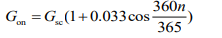
G_sc is the solar constant and equal to 1367 W/m2 and n is the day in the year. The term contained within cosine is in units degrees.

Brief Python Introduction

Packages and Calling Functions: In Python, there are several powerful computing packages commonly used that should be declared at the top of your .py, or python file. For example, some of the more popular computational packages useful for engineering include numpy, scipy, matplotlib and pandas, among others. These must be installed on your computer, either manually using a package installer (e.g. pip installer), or are installed by default with many Python distributions, including the Anaconda Distribution that we will use in this exercise. For example, if we want to utilize the numpy package we can use the import function and say:

which allows us to call the numpy package simply by typing np. If we wish to use numpy package to calculate the cosine of an angle, we would first need to call it by typing np followed by a period and then the function contained within the package we wish to utilize, in this case cos, and the value within it (in this case the numerical value pi which is also called using the numpy package as np.pi) contained within parenthesis. For example,

The input contained within parenthesis should have units radians and the output will be in units radians. For example, to correctly use the equation for Gon, the cosine term will look like the following.

because we need to convert from degrees to radians by multiplying everything by np.pi/180.

Declaring Functions: Functions are declared in Python by defining them using def followed by the function name, parenthesis that include any variables the function is dependent on, followed by a colon. The body of the function is then started on a new, indented line and the value that is returned by the function must be declared at the end using return. For example, if we wish to define a function y that depends on x and is a linear line with slope m and intercept y and later call it, we would write

 

Exercise
Complete the following questions that deal with determining G_on using the above equation and a more accurate form of the equation (not shown, Gon_accurate function), as a way to get comfortable computing in Python using some basic techniques, learning to call and declare functions, plotting data using the package matplotlib, and using two different methods to evaluate python code, namely a traditional editor named Spyder and a web based notebook style editor called Jupyter.

1. Download Python (“Anaconda Distribution”). This includes many useful packages but most commonly we will use Spyder and Jupyter, two different ways to evaluate Python code.
2. Open and run “Extraterrestrial Radiation Calculator.py” using Spyder. It can be copied and pasted from the appendix of this document and saved to your computer as a .py file. After running, you should see a plot with two curves.

   

3. Replot the data using the same code but change the plotted lines from red ‘r’ and blue ‘b’in the plt.plot lines of code, to other colors of your choice. Here are examples and more documentation .
4. We have plotted data every day using the function np.arrange with the linedays=np.arange(1,365,1). This creates an array from 1 to 365 with a spacing of 1.However, lets imagine we want to see individual data points plotted – it would be difficult to distinguish between them with so many. Therefore, lets plot a point every 10 days by changing the spacing from 1 to 10. Show the results using blue circles for the blue curve by inserting ‘bo’ in place of ‘b’.
5. Use Python Jupyter Notebook to the plot the extraterrestrial solar radiation (Gon) between March 1st and July 1st. Copy and paste lines from the prior “Extraterrestrial Radiation Calculator.py.py file”. You can group common lines of code in their own cells that can be evaluated independently from the remaining cells. At the end of that file are a few lines of code that you can use to determine the day in the year knowing a date. Adding a # sign at the beginning of each line is used to comment and is not evaluated. Copy and paste these lines into a new Jupyter cell to determine what days the required dates correspond to. For example, to determine the day in the year on March 1st see below. Thus the day on March 1st is 61 and July 1st is 183.

Now we will plot between only these days by changing days to equal  days=np.arange(61,183,1). Below is a screenshot of the cells and output.

Back to top

 

Exercise 2 Instructions

Solar Time

Solar time is used in all sun-angle relationships. It is based on the apparent angular motion of the sun across the sky, with solar noon the time the sun crosses the meridian of the observer. Two corrections are needed to convert from standard time.

1. Correction for difference in longitude between observer’s meridian and the meridian at which local standard time is based.
2. Correction from the equation of time which accounts for perturbations in the earth’s rate of rotation.

The equation used to calculate solar time is below.

L_st is the standard meridian for the local time zone, Lloc is the longitude of the location in question and E is the equation of time in minutes. E can be determined graphically from the figure below (from Duffie and Beckmann, Solar Engineering of Thermal Processes, 4th Edition) or from the equations below from Duffie and Beckmann (Duffie and Beckmann, Solar Engineering of Thermal Processes, 4th Edition).

Here, n is the day in the year and B has units degrees. The units for the right hand side of the equation used to calculate solar time are minutes.

To determine Lst, multiply the difference in time between local standard clock time and Greenwich Mean Time (GMT) by 15°. This relationship comes from thefact that the sun takes 4 minutes to traverse 1° of longitude. Thus, if your local standard clock is 1 hour behind GMT then LST is 15°. You must account for Daylight Savings Time (DST): for example, DST in the United States takes place between the dates of March 8th and November 1st. During this time, the clocks are advanced by 1 hour and thus the difference between the clocks in the United States and GMT changes by 1 hour. For example, if DST is 14:00 then Local Standard Time (LST) which should be used to determine solar time and Lst, is 13:00.

 

Figure 1. Equation of time verses month in the year. From Duffie and Beckmann, Solar Engineering of Thermal Processes, 4th Edition

Exercise
Find the instructions and full python code here. 

Back to top