Magnetohydrodynamics

INTRODUCTION

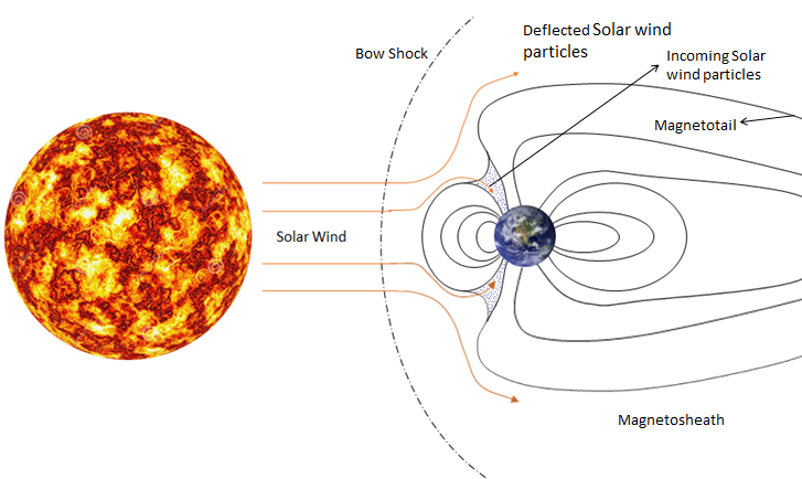
Magnetohydrodynamics (MHD) is governed by the laws of magnetism and Navier-Stokes equations. MHD flow can be found in both natural phenomena and man-made applications like solar wind (shown in figure above), sunspots, and interstellar clouds and for metallurgy and manufacturing. The most interesting phenomena in MHD flow is the interaction between the magnetic field and velocity field. Research on MHD became prominent with the discovery of Alfven waves which behave just like the transverse waves generated by a string in tension. However in MHD the magnetic field lines act as a string in which ions oscillate. Effect on conducting media in an imposed magnetic field can be explained using three vital processes. Firstly, the relative movement of conducting fluid in an imposed magnetic field will generate an electromotive force governed by the Faraday’s law and in turn this will generate electric currents. Secondly, these induced currents will give rise to magnetic field which will interact with the imposed field. Lastly, the induced and imposed field together will interact with the induced current and generate Lorentz force which will prevent the relative motion between the magnetic field and the fluid flow and thus it will appear as though the fluid is dragging the magnetic field lines with it.

 NUMERICAL METHOD

 A two dimensional fully parallelized time implicit Discontinuous Galerkin method has been implemented to solve for the ideal viscous MHD equations. The equations involve full Navier Stokes equations combined with the transient magnetic field equation and body forces generated due to the magnetic field. Various cases have been run to validate the inviscid as well as viscous part of this code, out of which two of the cases have been presented in Figure 1, Figure 2 and Figure 3. The inviscid part uses the Local Lax-Freidrich’s numerical flux. The viscous part of the code uses the Bassi and Rebay (BR2) [2] approach to get a more compact scheme and low memory requirement.

RESULTS

Orszag Tang Vortex

The Orszag Tang vortex problem gives an excellent insight on the evolution of Magnetohydrodynamic (MHD) turbulence in a compressible magnetofluid. MHD is governed by the laws of Magnetism and fluid flow. The orszag – tang is a test problem which shows how the imposed and induced field interact with each other and in turn generate shocks and contact discontinuities in the fluid flow. The existence of small scale structures in MHD are much stronger than the hydrodynamic counterpart. The compressibility creates massive jets in the domain which interact with each other and create eddies to generate a highly turbulent field.

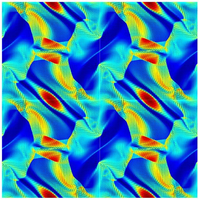
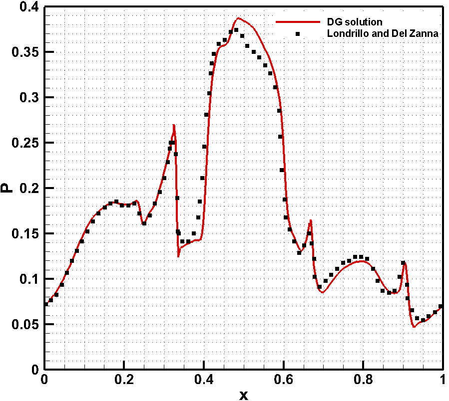
Figure 1: Density contour at time t=0.5 and pressure variation along y=0.4277 

The problem is initialized with nonrandom sinusoidal velocity and magnetic field and Figure 1 depicts the variation of the density in a periodic domain at time = 0.5. The simulation is carried out for P1 elements without any slope limiting or artificial diffusion. The divergence free condition of magnetic field is ensured by using Powell’s [3] eight wave formulation. The results shown in figure 1 are for the inviscid formulation of ideal MHD equations. The vectors shown are for the magnetic field and it clearly shows how the magnetic field interacts with the flow. The simulation is done on 256 × 256 uniform mesh and has been validated with the results presented by Londrillo & Del Zanna [4].

The results shown in figure 2 and figure 3 are for viscous MHD equations. They show the effect of compressibility on the velocity field as well as magnetic field. Figure 2(a) shows the velocity and figure 3(a) shows the magnetic field for M = 0.2 where compressibility effects are negligible. Figure 2(b) and Figure 3(b) shows the results for M = 0.6. Both the results shown are for time=2. The velocity streamlines show the significant effects of compressibility. Effect of compressibility on Magnetic streamlines is rather insignificant at this time. However as the simulation progresses the effects become more prominent on both magnetic field and velocities. The solutions have been validated using the results presented by Picone and Dahlburg [5].

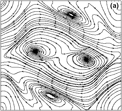
Figure 2: Velocity streamlines for (a) M = 0.2 (b) M = 0.6, showing how compressibility completely alters the velocity field at time = 0.2.

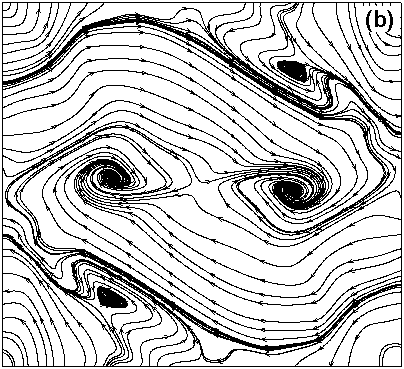
Figure 3:  Magnetic fieldlines for (a) M = 0.2 (b) M = 0.6, showing that compressiblity has a little effect on magnetic field at time  = 0.2.

REFERENCES

[1] P.A. Davidson, “An introduction to Magnetohydrodynamics”, Cambridge University Press, 2001

[2] Francesco Bassi, Andrea Crivellini, Stefano Rebay, Marco Savini, “Discontinuous Galerkin solution of the Reynolds-averaged Navier–Stokes and k–ω turbulence model equations”, Computers and Fluids, 34:507-540

[3] K. G. Powell, “An Approximate Riemann Solver for Magnetohydrodynamics (That Works in More Than One Dimension)”, Technical Report ICASE Report 94-24, ICASE, NASA Langley, 1994.

[4] P. Londrillo, L. Del Zanna, “High-Order Upwind Schemes for Multidimensional Magnetohydrodynamics”, the Astrophysical Journal, 530:508-524, 2000 February 10

[5] R. B. Dahlburg and J. M. Picone, “Evolution of the Orszag–Tang vortex system in a compressible medium. I. Initial average subsonic flow”, Phys. Fluids B 1(11), 2153 (1989).