The high-performance solver can be downloaded from GitHub.  The branch inverse has the acoustic simulation tool for generating a sound field around a polygon.

A sample command below is for loading the simulation program.  The parameters are based on above sketch. 

./main --obj_file="poly.obj" --src_type="point" --src_radi=4 --src_num=1 --oct_num=1\
--src_mag=1.0 --x_cnr=-2.56 --y_cnr=-2.56 --x_len=5.12 --y_len=5.12 --z_coord=0.5 --side_len=0.01\
--vox_file="vox1" --field_file="field"

obj_file: path for the obj object
src_type: type of sound source, "point" or "monopole"
src_radi: radius of source location
src_num: number of sources evenly distributed
oct_num: the number of octave bands, starting from 125 Hz or 2*pi*125 rad/s
src_mag: magnitude of sources
x_cnr: x coordinate of the corner of the simulation region
y_cnr: y coordinate of the corner of the simulation region
x_len: size of region in the x direction
y_len: size of region in the y direction
z_coord: z coordinate for the plane of interest, of the same height as the source
side_len: side length of a unit voxel
vox_file: the path of the file for the voxel grid
field_file: the path of the file for the loudness field
Viewing data: 
Generated data can be viewed using the MATLAB scirpt visualize_data.m in the MATLAB folder. 

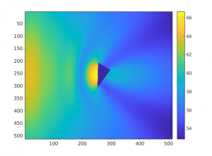
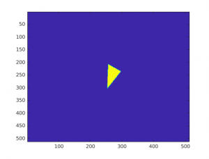
The outputs from visualize_data.m present two plots on x-y plan like below. One is for the sound field around the polygon, the other is for the voxelized plot of polygon on x-y section.